Example usages
This page contains two examples:
- a primary biliary cirrhosis (PBC) dataset, containing 7 clinical variables (age, sex, edema, bilirubin concentration, albumin concentration, prothrombin time, and disease stage) with 410 patients
- kidney renal cell carcinoma (KIRC) dataset using RNASeq gene expression data. Counts were normalized with DESeq2 and then log-ed (log2 + 1).
The PBC dataset was obtained from the "survival" package in R and the KIRC dataset was obtained from The Cancer Genome Atlas via the Broad Institute. Both datasets are standardized (mean = 0 and std. dev = 1) and located in the examples folder.
Plots were done in R rather than Python due to better support for plotting survival data.
PBC example
In this example, the L2 parameter is optimized using the L2CVProfile function, which cross validates the training data. A model is built using the trainCoxMlp function, and evalulated on the hold out test data.
from cox_nnet import *
import numpy
import sklearn

# load data
x = numpy.loadtxt(fname="PBC/x.csv",delimiter=",",skiprows=0)
ytime = numpy.loadtxt(fname="PBC/ytime.csv",delimiter=",",skiprows=0)
ystatus = numpy.loadtxt(fname="PBC/ystatus.csv",delimiter=",",skiprows=0)

# split into test/train sets
x_train, x_test, ytime_train, ytime_test, ystatus_train, ystatus_test = \
    sklearn.cross_validation.train_test_split(x, ytime, ystatus,
    test_size = 0.2, random_state = 100)

#Define parameters
model_params = dict(node_map = None, input_split = None)
search_params = dict(method = "nesterov", learning_rate=0.01, momentum=0.9,
    max_iter=2000, stop_threshold=0.995, patience=1000, patience_incr=2, rand_seed = 123,
    eval_step=23, lr_decay = 0.9, lr_growth = 1.0)
cv_params = dict(cv_seed=1, n_folds=5, cv_metric = "loglikelihood",
    L2_range = numpy.arange(-4.5,1,0.5))

#cross validate training set to determine lambda parameters
cv_likelihoods, L2_reg_params, mean_cvpl = L2CVProfile(x_train,ytime_train,ystatus_train,
    model_params,search_params,cv_params, verbose=False)
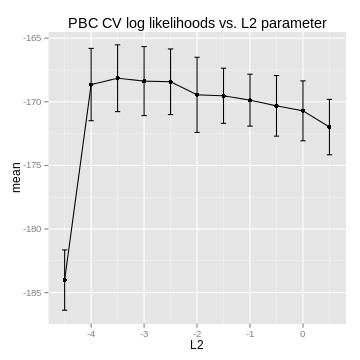
If you plot the data, you'll hopefully find a nice maximum to choose as the L2 parameter:
#Build the model
L2_reg = L2_reg_params[numpy.argmax(mean_cvpl)]
model_params = dict(node_map = None, input_split = None, L2_reg=numpy.exp(L2_reg))
model, cost_iter = trainCoxMlp(x_train, ytime_train, ystatus_train,
    model_params, search_params, verbose=True)
theta = model.predictNewData(x_test)
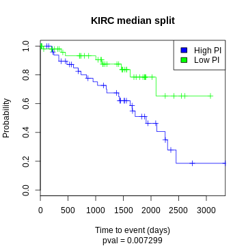
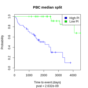
One common way to visualize a survival model is to split the test data by median log hazard ratio and plot the two curves:
KIRC example
In this example, the L2 parameter is optimized by a validation set (a subset of the training data) since cross-validation is computationally expensive. High throughput datasets should be run using multiple cores or the GPU. See: http://deeplearning.net/software/theano/tutorial/using_gpu.html
from cox_nnet import *
import numpy
import sklearn
# load data
x = numpy.loadtxt(fname="KIRC/log_counts.csv.gz",delimiter=",",skiprows=0)
ytime = numpy.loadtxt(fname="KIRC/ytime.csv",delimiter=",",skiprows=0)
ystatus = numpy.loadtxt(fname="KIRC/ystatus.csv",delimiter=",",skiprows=0)
# split into test/train sets
x_train, x_test, ytime_train, ytime_test, ystatus_train, ystatus_test = \
sklearn.cross_validation.train_test_split(x, ytime, ystatus, test_size = 0.2, random_state = 1)
# split training into optimization and validation sets
x_opt, x_validation, ytime_opt, ytime_validation, ystatus_opt, ystatus_validation = \
sklearn.cross_validation.train_test_split(x_train, ytime_train, ystatus_train,
test_size = 0.2, random_state = 1)
# set parameters
model_params = dict(node_map = None, input_split = None)
search_params = dict(method = "nesterov", learning_rate=0.01, momentum=0.9,
max_iter=2000, stop_threshold=0.995, patience=1000, patience_incr=2,
rand_seed = 123, eval_step=23, lr_decay = 0.9, lr_growth = 1.0)
cv_params = dict(cv_metric = "loglikelihood", L2_range = numpy.arange(-2,1,0.5))
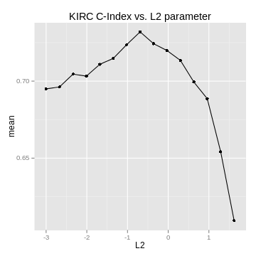
#profile log likelihood to determine lambda parameter
likelihoods, L2_reg_params = L2Profile(x_opt,ytime_opt,ystatus_opt,
x_validation,ytime_validation,ystatus_validation,
model_params, search_params, cv_params, verbose=False)
numpy.savetxt("KIRC_likelihoods.csv", likelihoods, delimiter=",")
#build model based on optimal lambda parameter
L2_reg = L2_reg_params[numpy.argmax(likelihoods)]
model_params = dict(node_map = None, input_split = None, L2_reg=numpy.exp(L2_reg))
model, cost_iter = trainCoxMlp(x_train, ytime_train, ystatus_train,
    model_params, search_params, verbose=True)
theta = model.predictNewData(x_test)
Interfacing and analysis with R
The preferred programming environment for many bioinformaticians is R. There are two ways to use Cox-nnet from R. 1) Using the rPython R package to interface with Cox-nnet (see http://rpython.r-forge.r-project.org/) or 2) calling Python scripts as a system call and reading the results in from the command line. The 2nd method is detailed below:
# Set Theano parameters
PARAMS = "THEANO_FLAGS=mode=FAST_RUN,device=gpu0,floatX=float32 %s"

# Call python script
system(sprintf(PARAMS,"examples/test_KIRC.py"))

# Read in the results on the test set
as.numeric(readLines("KIRC_theta.csv")) -> pred
as.numeric(readLines("KIRC_ytime_test.csv")) -> time
as.numeric(readLines("KIRC_ystatus_test.csv")) -> status

# Plot survival curves
library(survival)
split_r = as.numeric(pred > median(pred))
high_curve<-survfit(formula = Surv(time[split_r == 1],status[split_r == 1]) ~ 1)
low_curve<-survfit(formula = Surv(time[split_r == 0],status[split_r == 0]) ~ 1)
plot(high_curve,main="", xlab="Time to event (days)", ylab="Probability", col= "blue", conf.int=F, lwd=1, xlim=c(0, max(time)))
lines(low_curve, col= "green", lwd=1, lty=1, conf.int=F)
legend("topright", legend=c("High PI", "Low PI"), fill=c("blue","green"))